Audio Segmentation
Context
One of the most difficult tasks in speech processing is to define limits of the phonetic units present in the signal. Phones are strongly co-articulated and there are no clear borders among them, so the link between the linguistic and the acoustic segmentation is not simple to define. It does not matter which code level is chosen (word, syllable, phon): the acoustic variability of speech signal makes difficult all alignment efforts and its ambiguity challenges all proposed definitions.
Overview
We have developed an audio segmentation algorithm based on the acoustic signal level. If you are interested by python or C code, please contact us.
Forward backward segmentation
This segmentation is provided by the Forward-Backward Divergence algorithm, which is based on a statistical study of the acoustic signal.
Assuming that speech signal is described by a string of quasi-stationary units, each one is characterized by an auto regressive (AR) Gaussian model. The method consists in performing a detection of changes in AR models. Two AR models M0 and M1 are identified at every instant, and the mutual entropy between these conditionnal laws allows to quantify the distance between them. M0 represents the segment from last break in the signal while M1 is a short sliding window starting also after last break. When the distance between models change more than a certain limit, a new break is declared in the signal. The algorithm detects three sorts of segments: shorts or impulsive, transitory and quasi-stationary. We show here under an example of the segmentation where infra-phonetic units are determined.
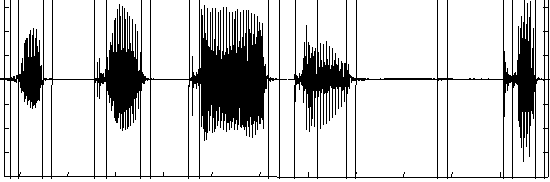
Results of speech segmenting algorithm
The use of an a priori segmentation partially removes redundancy for long sounds, and a segment analysis is relevant to locate coarse features. This approach have given interesting results in automatic speech recognition: experiments have shown that segmental duration carry pertinent information.
Contributors
- Régine André-Obrecht (contact)
- Patrice Pillot
- Julien Pinquier
- Maxime Le Coz
- Jérôme Farinas
7 Multilingual Phonetic Decoders Package
Package description
This package contains a set of 6 multilingual phonetic decoders: English, German, Hindi, Japanese, Mandarin and Spanish. Each decoder was trained on the Oregon Graduate Institute-Multi Language Telephone Speech Corpus.
The models are based on Hidden Model Markov. 10 Gaussians were used for each state. 12 PLP, the energy and their derivative were used for parametrerization. The frequency bank is in the range of the telephone speech: 300-3400 Hz. The overall topology of the models consists in 3 states HMM, with some adjustments considering the average acoustical duration of the phonetic class considered.
The labeling of each phoneme is based on the OGI labeling guide.
A script is provided in the package in order to facilitate the decoders handling. You will need the HTK toolkit installed in order to use it.
License
This package is free software; you can redistribute it and/or modify it under the terms of the GNU General Public License as published by the Free Software Foundation; either version 3 of the License, or (at your option) any later version.

Download (FTP)
- 6 multilingual decoders, version 1.2 (2008/10/06)
- 7 multilingual decoders, version 1.3 (2013/01/15) : adding of a French large band decoder
If you want to be involved with future development of this package, ask to by add to the user list: just send an email.
Please send any remark, enhancement to Jérôme Farinas
SAMOPLAY Demo
Context
Some of the most used SAMOVA algorithms could be tested live in the SAMOPLAY demonstration platform:
- Audio segmentation
- Speech identification
- Music identification
- Tempogram representation

Contributors
- Julien Pinquier
- Maxime Le Coz
- Jérôme Farinas
AESEG – Post-processing toolbox for the segmentation of times series
Context
During a sound event detection task, a speaker separation, or any time series segmentation task, the predictions at the output of a classification system can be unstable, and the segmentation is not necessarily obvious. There are then several ways to split these prediction curves into multiple segments.
The development of the AESEG library came spontaneously when we were confronted with the problem of segmentation of audio events in the context of my thesis, “Deep, semi-semi supervised learning for the classification and localization of sound events.” Which methods should we use? How to find the best segmentation parameters?
Overview
Audio Event SEGmentation (AESG) is a toolkit compiling a set of segmentation methods and optimization algorithms to delineate time series into discrete events. Written in python and accessible under the form of a package, and source code and documentation can be found here: https://github.com/aeseg/aeseg
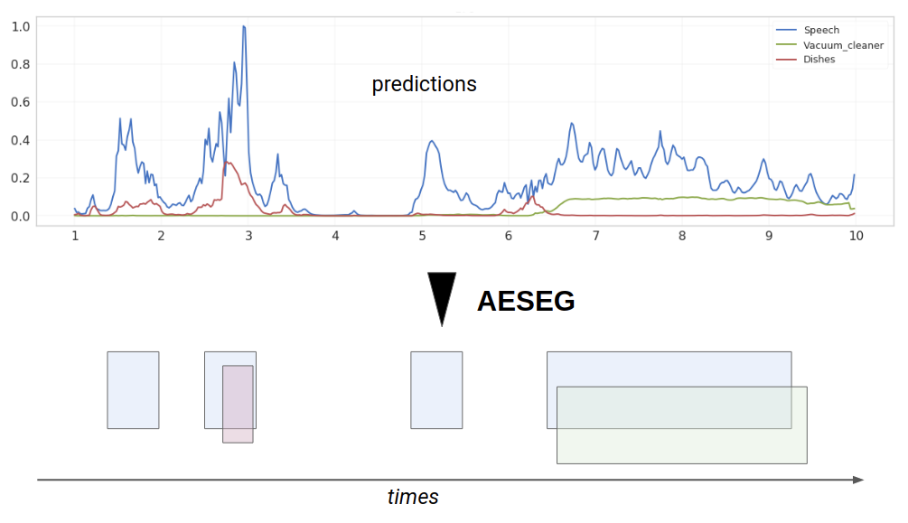
The output of prediction systems on temporal data is often used as-is, yet the data is often noisy, with a resolution too small to be used with confidence. A simple smoothing step can already improve the results of these systems. In the case of a classification system, the use of a fixed threshold is often insufficient. AESEG thus proposes a set of smoothing and thresholding methods combined with an optimization algorithm to select the best smoothing and thresholding parameters to maximize time prediction systems’ performance.
Segmentation algorithms
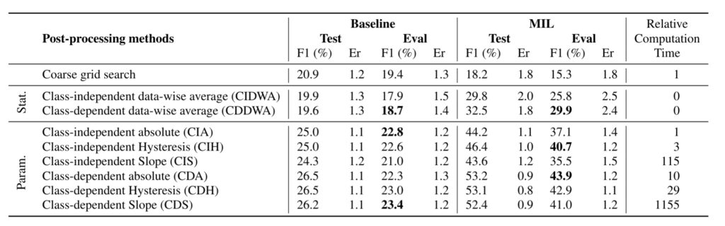
The seven available segmentation algorithms can be divided into two groups, the data-driven methods, and the parametric methods.
Data-driven methods
The statistics-based methods are directly based on the statistics extracted from the temporal predictions of each sample. The main advantage of these methods is that they are fast and often efficient.
By directly using the system temporal predictions, the mean is computed and used as a segmentation threshold. Depending on the methods used, the calculation of the average can be done either at the file or dataset level. Moreover, it can also be independent or dependent on the class (the median can also be used).
- Class-independent data-wise average: The average is computed using the temporal prediction from the whole dataset and the classes.
$$ \forall x \in S, Th=\frac{1}{N}\sum p(x) $$ - Class-independent file-wise average: n is the size of the prediction from one file. It depends on the precision of the system.
$$\forall x \in S, Th_x= \frac{1}{n} \sum p(x)$$ - Class-dependent data-wise average: c represent the class and C the ensemble of class the system can target.
$$\forall x \in S, \forall c \in C, Th_c = \frac{1}{N} \sum p_c(x)$$ - Class-dependent file-wise average: c represent the class and C the ensemble of class the system can target. n is the size of the prediction from one file. It depends on the precision of the system.
$$\forall x \in S, \forall c \in C, Th_{xc} = \frac{1}{n} \sum p_c(x)$$
Parametric methods
These methods optimize the segmentation parameters using the dichotomous search or genetic algorithms. The three images below describe the different algorithms currently available.
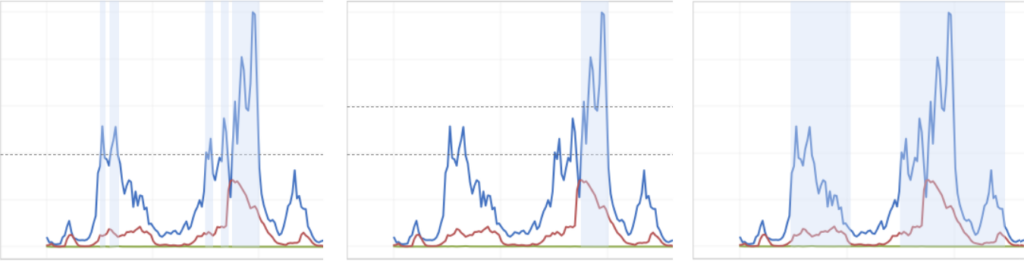
Absolute thresholding
Absolute thresholding refers to applying a unique and arbitrary threshold to the temporal predictions without using their statistics. This naive approach still yields exploitable results that can get close to the best ones in some cases. It is also the approach with the shortest optimization time due to the unique parameter to optimize. Every probability above this threshold will count as a valid part of the segment.
Hysteresis thresholding
The hysteresis threshold is used in many fields, such as finance, imaging, electronics, etc. It is a simple method to implement and has proven itself many times over. This method is based on two thresholds. One is used to determine the beginning of a segment and the other (smaller) its end. This algorithm is used when probabilities are unstable and changing at a high pace. It should, therefore, decrease the number of events detected by the algorithm and reduce the insertion and deletion rates, giving a better error rate than the Absolute threshold approach.
Edge thresholding
Called slope in the toolkit, this method determines the start and end of a segment by detecting a fast change in the probabilities over time. Fist-rising values imply the beginning of a segment while fast decreasing values followed by a plateau imply the end of the segment. This method makes it possible to obtain a single segment from an event repeated several times over a short period, diminishing the final number of small segments.
Optimization algorithm
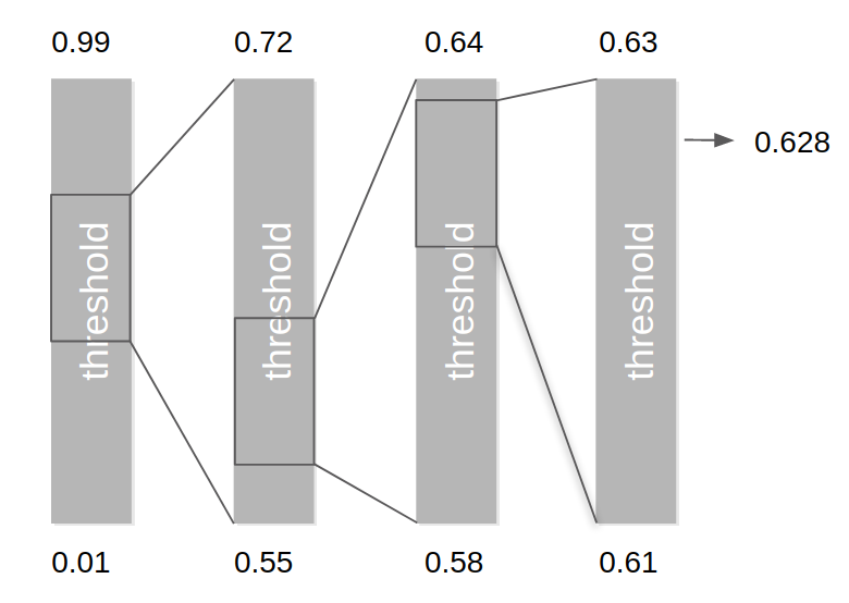
The parametric methods regroup together the different algorithms that exploit arbitrary parameters to perform the segmentation. Depending on the number of parameters to tune, the search space growth is exponential and execution time will often exceed reasonable times. The dichotomous search algorithm implemented in AESEG greatly reduce the number of combination to be tested. The user provides the initial search interval for each parameter that needs to be optimized, the optimization system will then start every combination using a coarse resolution. The best value for each parameter is selected and a new – shorter – interval computed around these new values. The process is repeated several times, each time increasing the precision of the final result.
Application on Sound Event Detection system
This work was initially developed for the DCASE 2018 – task 4 competition which provides 10 seconds audio files. Each of them could include one or several audio events from a set of 10 sound classes. The task was to provide a list of segments correctly delimiting each event contained in these files. AESEG was applied to the output of a temporal classifier to extract sound events under segments. Using AESEG allows us to gain up to 28 points, confirming the importance of good post-processing.
Contributor
Léo Cances, Thomas Pellegrini, Patrice Guyot
Projects
LUDAU – Lightly-supervised and Unsupervised Discovery of Audio Units using Deep Learning
Main publication
- L. Cances, P. Guyot and T. Pellegrini, “Evaluation of Post-Processing Algorithms for Polyphonic Sound Event Detection,” 2019 IEEE Workshop on Applications of Signal Processing to Audio and Acoustics (WASPAA), New Paltz, NY, USA, pp. 318-322, doi: 10.1109/WASPAA.2019.8937143.
- L. Cances, T. Pellegrini, P. Guyot, “Mutli Task Learning and Post Processing Optimization for Sound Event Detection,” 2019 Detection and Classification of Acoustic Scenes and Events (DCASE) Challenge, New York, NY, USA.
Reference
- X. Xia, R. Togneri, F. Sohel, and D. Huang, “Frame-wise dynamic threshold based polyphonic acoustic event detection,” inProc. Interspeech, Stockholm, 2017, pp.474–478. [Online]. Available:http://dx.doi.org/10.21437/Interspeech.2017-746
- Q. Kong, I. Sobieraj, W. Wang, and M. Plumbley, “Deep neu-ral network baseline for DCASE challenge 2016,” Budapest,2016.
- J. Salamon, B. McFee, P. Li, and J. P. Bello, “Multiple in-stance learning for sound event detection,” DCASE Chal-lenge, Munich, Tech. Rep., 2017.
- A. Mesaros, T. Heittola, T. Virtanen, A. Mesaros, T. Heittola,and T. Virtanen, “Metrics for Polyphonic Sound EventDetection,”Applied Sciences, vol. 6, no. 6, p. 162, May2016. [Online]. Available: http://www.mdpi.com/2076-3417/6/6/162
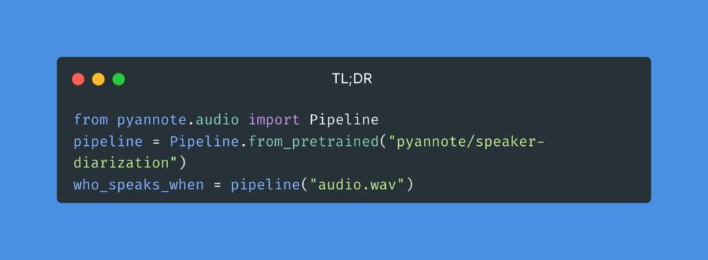
Speaker diarization with pyannote.audio
Speaker diarization is the process of partitioning a multi-party conversation into homogeneous temporal segments according to the identity of the speaker. In contrast with speaker verification, identification, detection or even tracking, speaker diarization does not assume prior enrollment of speakers: the number and identity of speakers are usually not known a priori.
As such, it can be seen as an unsupervised machine learning task analogue to clustering. One has to segment and tag all speech regions of the same speaker with the same label — though neither the actual pool of labels nor their order is important (i.e. 1 – 2 – 3 – 2 – 3 is the same as A – B – C – B – C or 2 – 3 – 1 – 3 – 1.).

It is usually addressed by putting together a collection of building blocks, each tackling a specific sub-task, in sequence:
- Voice activity detection is the task of detecting speech regions in a given audio stream or recording.
- Speaker change detection is the task of detecting speaker change points in a given audio stream or recording.
- Clustering is the task of grouping speech turns according to the speaker identity.
- Overlapped speech detection is the task of detecting regions where at least two speakers are speaking at the same time.
- Resegmentation is the task of refining speech turn boundaries and labels. It is usually applied as a final post-processing step of a speaker diarization pipeline.
pyannote.audio is an open-source deep learning toolkit developed by Hervé Bredin since 2010 that allows to both perform speaker diarization based on shared pretrained models and adapt existing models to specific domains.
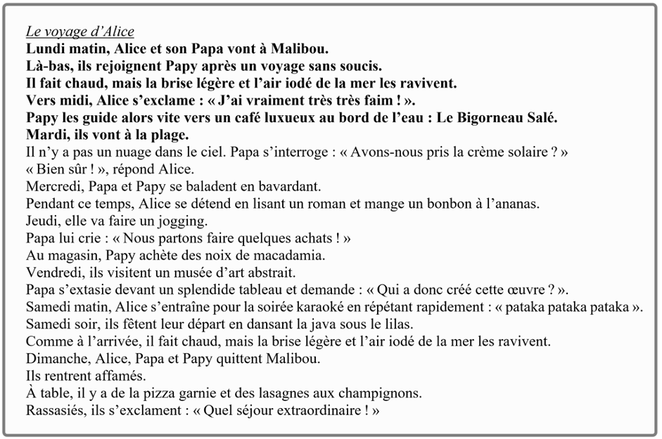
Le voyage d’Alice
Extraction automatique de mesures acoustiques de la parole et de la voix sur une lecture à voix haute du texte standardisé
Contributeurs
- Timothy Pommée (timothy_pommee@hotmail.com) : https://orcid.org/0000-0001-7846-7282
- Liziane Bouvier : https://orcid.org/0000-0002-7239-7639
- Julien Pinquier : https://orcid.org/0000-0003-1556-1284
- Julie Mauclair : https://orcid.org/0000-0002-2740-5118
- Véronique Delvaux : https://orcid.org/0000-0002-4200-2982
- Cécile Fougeron : https://orcid.org/0000-0002-2166-4602
- Corine Astésano : https://orcid.org/0000-0002-0882-4974
- Vincent Martel-Sauvageau : https://orcid.org/0000-0003-0152-0908
- Dominique Morsomme : https://orcid.org/0000-0002-7697-0498
- Muriel Lalain : https://orcid.org/0000-0002-7672-8589
- Virginie Woisard : https://orcid.org/0000-0003-3895-2827
- Pierre Pinçon
Publication
Pommée, T., Pinquier, J., Mauclair, J., Bouvier, L., Delvaux, V., Fougeron, C., Astésano, C., Martel-Sauvageau, V., Morsomme, D., Pinçon, P., Lalain, M., & Woisard, V. (2023). Le voyage d’Alice : un texte standardisé pour l’évaluation de la parole et de la voix en Français. Glossa, XXX.
Introduction
Le texte “Le voyage d’Alice” a été créé spécifiquement pour l’évaluation de la parole et de la voix en français, sur base d’un ensemble exhaustif de critères, prenant en compte les données de la littérature, les besoins spécifiques identifiés en recherche scientifique et en pratique clinique francophone, ainsi que les données d’une étude de consensus internationale. Sa construction est décrite en détails et en français dans la publication dont la référence est renseignée ci-dessus.
Ce texte est destiné à fournir un support standardisé pour l’évaluation :
- de l’articulation des sons de la parole (dysarthrie, apraxie) ;
- des variations prosodiques et du comportement phonatoire (dysphonie, harmonisation vocale) ;
- de la fluence/des disfluences (bégaiement/bredouillement) ;
chez les locuteurs âgés d’au moins 12 ans.
Il s’est montré utilisable et facilement lisible en Belgique, en France comme au Canada.
Le texte standardisé
Instructions et installation
Pour en savoir plus, voici un document explicatif avec le code…