Practical: Generalized Hough Transform

The purpose of this practical is to implement the complete procedure for modeling and recognition of the generalized Hough transform in matlab.
Some algorithms are given to simplify the exercise.

I. Basic functions

Initially, you will need to prepare a set of function that will be used thereafter.

I.1 "contour" function

Copy the contour.m function (click on the link).
This function allows you to retrieve a list of points on the contour of a shape contained in an binary image. The function parameter (income variable) is a 2D matrix containing only 0 and 1.
Display and understand the values of the outcome variable "contour_list".

I.2 "beta" function

Copy the beta.m function (click on the link).
This function allows you to retrieve the angle value from the perpendicular to the tangent inside of the shape at a given contour point.
Determine the expected values in entry for this function and their role.

I.3 "barycenter" function

Write the "barycenter.m" function which computes and returns the gravitational center coordinates of a shape (contained in a binary image, passed as parameter):
[xo,yo]=barycenter(img)

I.4 "alpha" function

Copy the alpha.m function (click on the link).
This function allows to retrieve the angle value between the line connecting each contour points and the gravitational center to the x-axis.
Determine the expected values in entry for this function and their role.

I.5 "distance" function

Write the "distance.m" function which computes and returns the Euclidean distance between two points which coordinates are passed as parameters:
d=distance(x1,y1,x2,y2)

II. Modeling

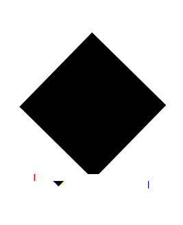
We will produce the "model" of this form, against the purposes of the Generalized Hough Transform.
To do this, complete the function below: parts with "...".
To have more information, do not forget to read the comments.

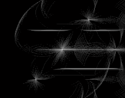
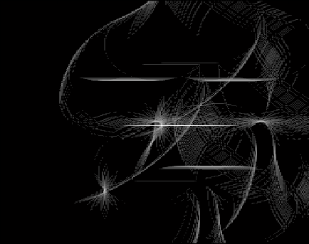
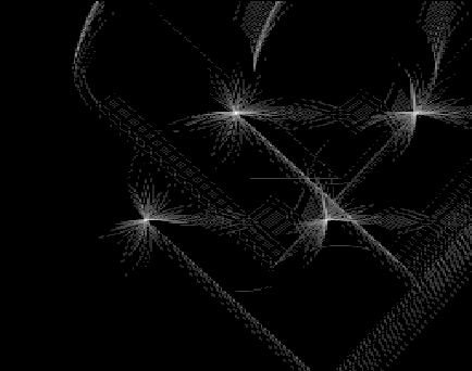
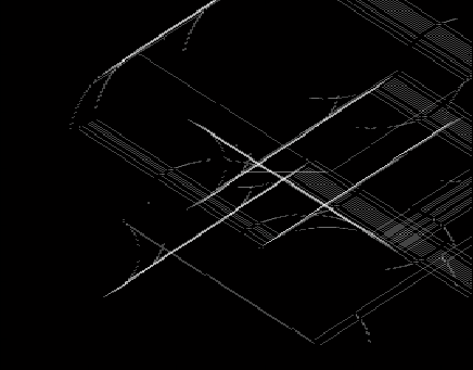
function [H]=ModelHough(imgRGB)
% Generalized Hough Transform Modeling

% Image Binarization
...

% Retrieving information about the contour: points and number (N)
...

% Model initialization:
    % row = beta value * 100
    % column = number of the couple (alpha, distance)
    % 3rd dimension: 1 = alpha, 2 = distance
H=zeros(round(100*2*pi),N,2);

% Compute of the barycenter coordinates
...

% for each contour point
for i=1:N

    % beta compute for i^th contour point
    b=...

    % research of the first column
    k=1;
    while H(b+1,k,2)~=0
       k=k+1;
    end

    % compute of the alpha value
    H(b+1,k,1)=...

    % compute of the distance value
    H(b+1,k,2)=...

end

III. Recognition

We will now apply the recognition process using the previous modeling (section II).
Produce voting space corresponding to each of 4 forms given below: an example is given for each image.

To display the voting space V (like a image), use the following instructions:
imagesc(log(V+1));
colormap(gray(256));

Check that the image of the model is one that produces the highest vote in the produced voting spaces.

Binary image	Voting space