Bayesian estimation of multifractal parameters for multivariate time series: basics.

In this brief tutorial, we will step by step perform the multifractal analysis of a collection of time series that have been collected by regularly spaced sensors in a plane, using Bayesian estimators for the multifractal parameters (log-cumulants) c2 and c1.

Preliminaries and input data
Univariate (independent) analysis of the data components using non-informative priors
Multivariate analysis of the time series with regularizing joint priors
Time-localized multivariate analysis
Time-localized multivariate analysis using overlapping analysis windows

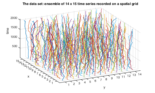
Preliminaries and input data

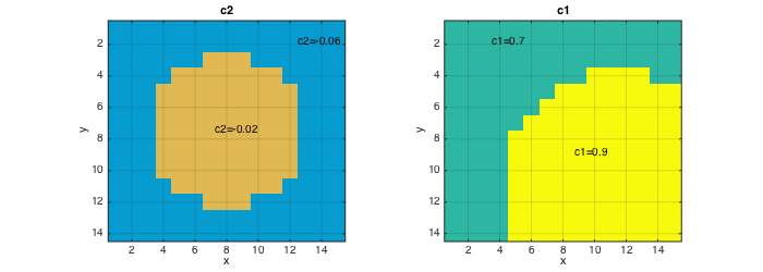
To begin with, set the path to the toolbox, load the data set (situated in this folder), and display it. The time series are independent realization of multifractal random walks with prescribed values for c1 and c2 that vary in space.

% add path to toolbox
clear all; clc;
currentpath = cd;addpath([currentpath(1:end-5)]);addpath([currentpath(1:end-5) '/all_tools/']);


% load synthetic data
load('demo_TS_2.mat'); k = 2; data = squeeze(data(:,:,k,:));
c2 = c2(:,:,k);C2T=unique(c2);c1 = c1(:,:,k);C1T=unique(c1); C1 = [0.6 0.8]; C2 = [-0.09 0];

% display data and theoretical values for c2 and c1
zdata=zscore(data,0,3)/4;
figure(1);clf;hold on;set(gcf,'position',[10 500 500 300]);
for k1=1:size(data,1); for k2=1:size(data,2);
        plot3(squeeze(zdata(k1,k2,:))+k1-squeeze(zdata(k1,k2,1)), ...
            k2+zeros(size(squeeze(zdata(k1,k2,:)))), 1:length(squeeze(zdata(k1,k2,:))));
    end;end
title('The data set: ensemble of 14 x 15 time series recorded on a spatial grid');zlabel('time');xlabel('y');ylabel('x');grid on;
set(gca,'zlim',[1 2^11]);axis([0 15 0 16 1 2^11]);set(gca,'xtick',[1:14]);set(gca,'xticklabel',[1:14]);
set(gca,'ytick',[1:15]);set(gca,'yticklabel',[1:15]);view([-26,36]);

figure(2);clf; set(gcf,'position',[10 10 700 250]);
subplot(121);imagesc(c2);axis image; grid on; caxis(C2); title('c2');xlabel('x');ylabel('y');
hold on; text('string',['c2=',num2str(C2T(1))],'units','normalized','pos',[0.8 0.9]);
hold on; text('string',['c2=',num2str(round(C2T(2)*100)/100)],'units','normalized','pos',[0.45 0.5]);
subplot(122);imagesc(c1);axis image; grid on; caxis(C1); title('c1');xlabel('x');ylabel('y');
hold on; text('string',['c1=',num2str(C1T(1))],'units','normalized','pos',[0.2 0.9]);
hold on; text('string',['c1=',num2str(round(C1T(2)*100)/100)],'units','normalized','pos',[0.55 0.4]);

Univariate (independent) analysis of the data components using non-informative priors

We perform the univariate (i.e., component-by-component) multifractal analysis of the data set using standard linear regression based estimation and Bayesian estimation with non-informative (univariate) priors.

% First we need to fix the parameters of the multifractal analysis.

% Multifractal analysis parameters
Nwt = 2;    % number of vanishing moments of wavelet (Daubechies)
gamint = 0; % fractional integration parameter for wavelet leaders
j1=3;       % scaling range lower cutoff
j2=7;       % scaling range upper cutoff

We also need to determine how the data set is analyzed. Since the data comes in form of a cube (of size Nx x Ny x Nt), we need to tell the algorithms that this is not to be treated as a series of images (of size (Nx x Ny), but as a set of time series (of length Nt). This is done with the parameter "sw" (time analysis window length). The additional parameter "dsw" enables to define an overlap between time analysis windows (see below).

% data handling parameters
sw=size(data,3);  % time window length to be analyzed (here, the entire time series)
dsw=0*sw;       % overlap of time series windows (here, there is only one window per series)

These set of parameters (j1,j2,Nwt,gamint,sw,dsw) is all that must be specified by the user. We will see later how to change values of other relevant variables that are automatically set to default values when using only this minimal specification.

The analysis is performed in three steps:

The function "preproc_data_mvmfa" cuts the data set into its components according to our specification (sw,dsw), i.e., here, into its constituting time series, computes the wavelet leaders and the DFT of their logarithm, which is output in "lxft". "lxft" is the input data for the Bayesian estimation algorithms. The second output "param_data" contains parameters associated with "lxft".
The function "init_model_mvmfa" precomputes fixed terms in the Bayesian model and initializes the prior parameters, which are output in "param_model".
The actual Bayesian estimation is performed by the function "est_bayes_mvmfa". It approximates the MMSE estimators for the parameters c2, c1 using a Gibbs sampler (the other outputs will be discussed later).

For comparison, we also compute standard linear regression based estimates for c1 and c2 using the function "linfit_cp".

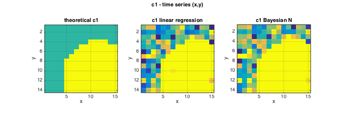
% Data cutting and computation of DWT and DFT
[lxft,param_data] = preproc_data_mvmfa(data,sw,dsw,j1,j2,Nwt,gamint);
% Precomputation of fixed terms initialization of prior parameters in the Bayesian model
[param_model] = init_model_mvmfa(param_data);

% Bayesian estimation for (c1,c2)
[ec2{2},~,~,~,ec1{2}] = est_bayes_mvmfa(lxft,param_model);

% Linear regression based estimation (for comparison)
[ec2{1},ec20{1},ec1{1},ec10{1}] = linfit_cp(param_data,0);

% plot the results
figure(2);clf; set(gcf,'position',[10 10 700 250]);
subplot(131);imagesc(squeeze(c2));axis image; grid on; caxis(C2); title('theoretical c2');xlabel('x');ylabel('y');
subplot(132);imagesc(squeeze(ec2{1}));axis image; grid on; caxis(C2); title('c2 linear regression');xlabel('x');ylabel('y');
subplot(133);imagesc(squeeze(ec2{2}));axis image; grid on; caxis(C2); title('c2 Bayesian IG');xlabel('x');ylabel('y');
axes('Units','Normal');h = title('c2 - time series (x,y)');set(gca,'visible','off');set(h,'visible','on');

figure(3);clf; set(gcf,'position',[1000 10 700 250]);
subplot(131);imagesc(squeeze(c1));axis image; grid on; caxis(C1);title('theoretical c1');xlabel('x');ylabel('y');
subplot(132);imagesc(squeeze(ec1{1}));axis image; grid on; caxis(C1); title('c1 linear regression');xlabel('x');ylabel('y');
subplot(133);imagesc(squeeze(ec1{2}));axis image; grid on; caxis(C1); title('c1 Bayesian N');xlabel('x');ylabel('y');
axes('Units','Normal');h = title('c1 - time series (x,y)');set(gca,'visible','off');set(h,'visible','on');

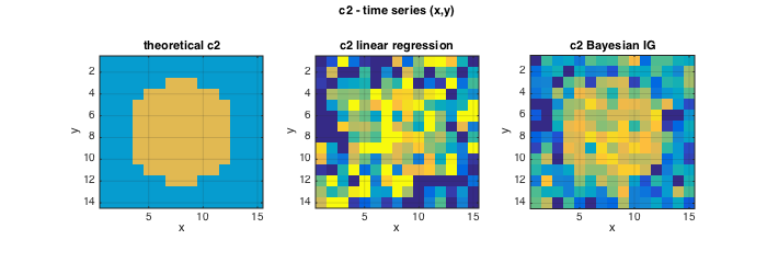
Note that the values output by the Bayesian estimator will slightly vary each time the estimator is re-run, despite the fact that the the data remain the same. This is to be expected since the Gibbs sampler is a stochastic algorithm that approximates the posterior expectation by the average of samples drawn at random from the posterior distribution.

Also note that the Bayesian estimator for c2 significantly improves estimation quality over the standard linear regression based estimation.

For c1, the estimates for linear regression and Bayesian estimation are identical because the non-informative Normal prior leads to an estimator equivalent to a linear regression.

Multivariate analysis of the time series with regularizing joint priors

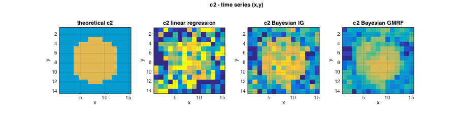
The estimation performance of the Bayesian estimator for multivariate data, such as a collection of time series, can be significantly improved by using informative, regularizing joint priors for the parameters c2 and c1 of the data components. The following priors are used for c2 and c1:

The prior for c2 is constructed as a hidden gamma Markov random field (GMRF). For the image patches considered here, a spatial (2D) prior is used. The degree of regularization induced by the prior is determined by hyperparameters that must be specified.

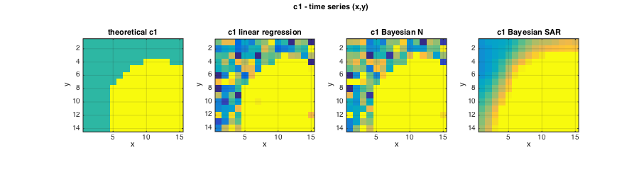
The prior for c1 is a Gaussian-type simultaneous autoregression (SAR) prior. The hyperparameters that tune the degree of regularization are embedded in the Bayesian model and automatically estimated.

Before performing the estimation, we adjust the hyperparameter of the GMRF. The hyperparameter for the 2D GMRF can be changed from the default value as follows:

% adjust regularization parameter for 2D GMRF prior for c2
param_model.EST.GMRF.a = 8 * ones(size(param_model.EST.GMRF.a));

The informative priors GMRF and SAR are activated by the additional input [GMRF SAR] to est_bayes_mvmfa, where GMRF and SAR are 1 or 0 (for on or off). For example, [0 0] will perform univariate estimation as above, [1 1] will perform joint estimation using GMRF for c2 and SAR for c1, [1 0] will use the informative (GMRF) prior for c2 and univariate priors for c1, and the combination [0 1] is not implemented.

% Perform joint estimation for (c2,c1) using informative GMRF and SAR priors
REGU=[1 1]; [ec2{3},Tc2,ec20tp,Tc20,ec1{3},Tc1,ec10tp,Tc10] = est_bayes_mvmfa(lxft,param_model,REGU);

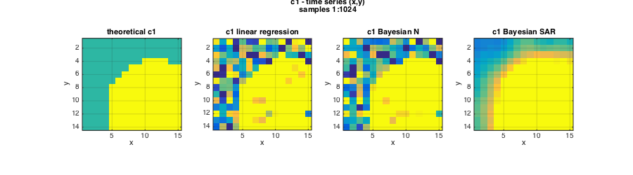
The following plots illustrate that the informative GMRF prior further improves the estimation performance for c2, and that now also the Bayesian estimation of c1 clearly improves over linear regression based estimates.

% Plots
figure(2);clf; set(gcf,'position',[10 10 900 250]);
subplot(141);imagesc(squeeze(c2));axis image; grid on; caxis(C2); title('theoretical c2');xlabel('x');ylabel('y');
subplot(142);imagesc(squeeze(ec2{1}));axis image; grid on; caxis(C2); title('c2 linear regression');xlabel('x');ylabel('y');
subplot(143);imagesc(squeeze(ec2{2}));axis image; grid on; caxis(C2); title('c2 Bayesian IG');xlabel('x');ylabel('y');
subplot(144);imagesc(squeeze(ec2{3}));axis image; grid on; caxis(C2); title('c2 Bayesian GMRF');xlabel('x');ylabel('y');
axes('Units','Normal');h = title('c2 - time series (x,y)');set(gca,'visible','off');set(h,'visible','on');
figure(3);clf; set(gcf,'position',[700 10 900 250]);
subplot(141);imagesc(squeeze(c1));axis image; grid on; caxis(C1);title('theoretical c1');xlabel('x');ylabel('y');
subplot(142);imagesc(squeeze(ec1{1}));axis image; grid on; caxis(C1); title('c1 linear regression');xlabel('x');ylabel('y');
subplot(143);imagesc(squeeze(ec1{2}));axis image; grid on; caxis(C1); title('c1 Bayesian N');xlabel('x');ylabel('y');
subplot(144);imagesc(squeeze(ec1{3}));axis image; grid on; caxis(C1); title('c1 Bayesian SAR');xlabel('x');ylabel('y');
axes('Units','Normal');h = title('c1 - time series (x,y)');set(gca,'visible','off');set(h,'visible','on');

Time-localized multivariate analysis

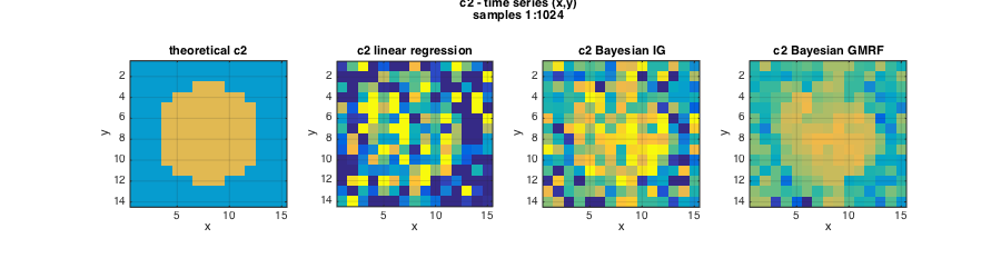
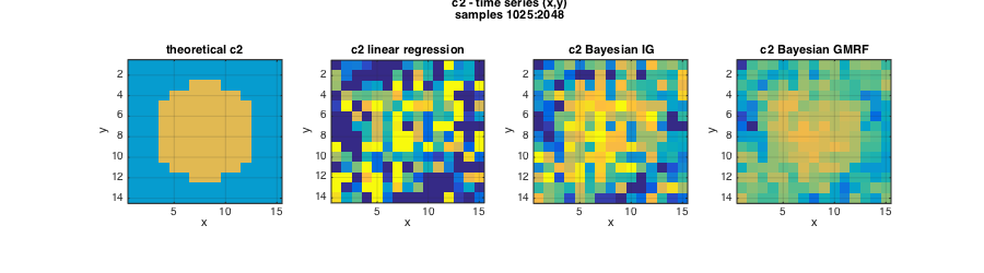
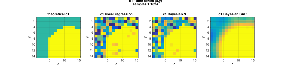
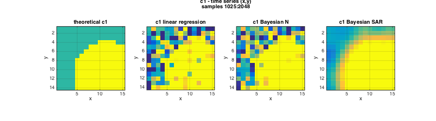
As shown above, we can use the multivariate nature of the data set to regularize estimation in a Bayesian estimation framework, permitting to reduce the variability of the estimates. This can also be used to regularize time-localized (via analysis windows) estimation. We only show the principle here by analyzing the first and last half of the time series.

sw=size(data,3)/2;  % time window length to be analyzed: first and second half
dsw=0*sw;       % overlap of time series windows (here, none)

Since time (multifractal analysis direction) and space (sensor placement) have physically very different roles, it makes sense to use the anisotropic prior "2D+1D" that has a different structure for the spatial and the temporal component. It is activated by passing the tag '2D+1D' as an additional input to "est_bayes_mvmfa.m"

% adjust regularization parameters for 2D+1D GMRF prior for c2
param_model.EST.GMRF.a = 4 * ones(size(param_model.EST.GMRF.a)); % spatial component
param_model.EST.GMRF.b = 4 * ones(size(param_model.EST.GMRF.b)); % temporal component
tag='2D+1D'; % anisotropic 2D prior

% Data cutting and computation of DWT and DFT
[lxft,param_data] = preproc_data_mvmfa(data,sw,dsw,j1,j2,Nwt,gamint);
% Precomputation of fixed terms initialization of prior parameters in the Bayesian model
[param_model] = init_model_mvmfa(param_data);
% Bayesian estimation for (c2,c1) using informative GMRF and SAR joint priors
REGU=[1 1]; [ec2{3},Tc2,ec20tp,Tc20,ec1{3},Tc1,ec10tp,Tc10] = est_bayes_mvmfa(lxft,param_model,REGU);
% Linear regression based estimation (for comparison)
[ec2{1},ec20{1},ec1{1},ec10{1}] = linfit_cp(param_data,0);
% Bayesian estimation for (c1,c2) with non-informative, univariate priors (for comparison)
[ec2{2},~,~,~,ec1{2}] = est_bayes_mvmfa(lxft,param_model);

% Plots
figure(2);clf; set(gcf,'position',[10 10 900 250]);
subplot(141);imagesc(squeeze(c2));axis image; grid on; caxis(C2); title('theoretical c2');xlabel('x');ylabel('y');
subplot(142);imagesc(squeeze(ec2{1}(:,:,1)));axis image; grid on; caxis(C2); title('c2 linear regression');xlabel('x');ylabel('y');
subplot(143);imagesc(squeeze(ec2{2}(:,:,1)));axis image; grid on; caxis(C2); title('c2 Bayesian IG');xlabel('x');ylabel('y');
subplot(144);imagesc(squeeze(ec2{3}(:,:,1)));axis image; grid on; caxis(C2); title('c2 Bayesian GMRF');xlabel('x');ylabel('y');
axes('Units','Normal');h = title({'c2 - time series (x,y)', 'samples 1:1024'});set(gca,'visible','off');set(h,'visible','on');
figure(4);clf; set(gcf,'position',[10 300 900 250]);
subplot(141);imagesc(squeeze(c2));axis image; grid on; caxis(C2); title('theoretical c2');xlabel('x');ylabel('y');
subplot(142);imagesc(squeeze(ec2{1}(:,:,2)));axis image; grid on; caxis(C2); title('c2 linear regression');xlabel('x');ylabel('y');
subplot(143);imagesc(squeeze(ec2{2}(:,:,2)));axis image; grid on; caxis(C2); title('c2 Bayesian IG');xlabel('x');ylabel('y');
subplot(144);imagesc(squeeze(ec2{3}(:,:,2)));axis image; grid on; caxis(C2); title('c2 Bayesian GMRF');xlabel('x');ylabel('y');
axes('Units','Normal');h = title({'c2 - time series (x,y)', 'samples 1025:2048'});set(gca,'visible','off');set(h,'visible','on');

figure(3);clf; set(gcf,'position',[700 10 900 250]);
subplot(141);imagesc(squeeze(c1));axis image; grid on; caxis(C1);title('theoretical c1');xlabel('x');ylabel('y');
subplot(142);imagesc(squeeze(ec1{1}(:,:,1)));axis image; grid on; caxis(C1); title('c1 linear regression');xlabel('x');ylabel('y');
subplot(143);imagesc(squeeze(ec1{2}(:,:,1)));axis image; grid on; caxis(C1); title('c1 Bayesian N');xlabel('x');ylabel('y');
subplot(144);imagesc(squeeze(ec1{3}(:,:,1)));axis image; grid on; caxis(C1); title('c1 Bayesian SAR');xlabel('x');ylabel('y');
axes('Units','Normal');h = title({'c1 - time series (x,y)', 'samples 1:1024'});set(gca,'visible','off');set(h,'visible','on');
figure(5);clf; set(gcf,'position',[700 300 900 250]);
subplot(141);imagesc(squeeze(c1));axis image; grid on; caxis(C1);title('theoretical c1');xlabel('x');ylabel('y');
subplot(142);imagesc(squeeze(ec1{1}(:,:,2)));axis image; grid on; caxis(C1); title('c1 linear regression');xlabel('x');ylabel('y');
subplot(143);imagesc(squeeze(ec1{2}(:,:,2)));axis image; grid on; caxis(C1); title('c1 Bayesian N');xlabel('x');ylabel('y');
subplot(144);imagesc(squeeze(ec1{3}(:,:,2)));axis image; grid on; caxis(C1); title('c1 Bayesian SAR');xlabel('x');ylabel('y');
axes('Units','Normal');h = title({'c1 - time series (x,y)', 'samples 1025:2048'});set(gca,'visible','off');set(h,'visible','on');

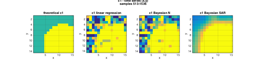
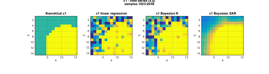
Time-localized multivariate analysis using overlapping analysis windows

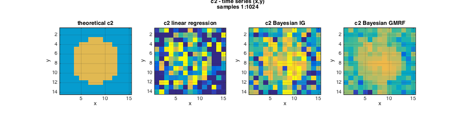
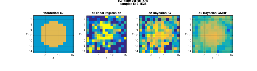
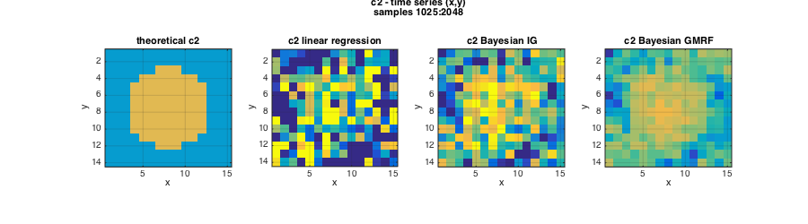
Finally, the analysis can be further localized by permitting the analysis windows overlap, as illustrated below with an overlap of 50% (i.e., adding a middle segment to the previous analysis)