Bayesian estimation of multifractal parameters: Output structures

We detail the format and meaning of the optional outputs of the main functions of the toolbox.

Synthetic image data
Optional outputs of data preprocessing function "preproc_data_mvmfa.m"
Outputs of Bayesian estimator / Gibbs sampler "est_bayes_mvmfa.m"

Synthetic image data

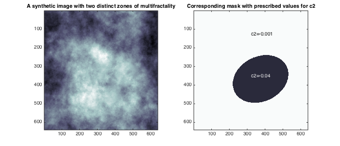
The image used here for illustration is a realization of a random field with controlled multifractal properties: c1 is constant and equals c1=0.7, and c2 takes the values c2=-0.04 in side an elliptical region, and c2=-0.001 outside.

% add path to toolbox and load synthetic image
clear all; clc;
currentpath = cd;addpath([currentpath(1:end-5)]);addpath([currentpath(1:end-5) '/all_tools/']);
load('MRWseries640_6.mat'); data=squeeze(data(:,:,5));
C1T=C1;C2T=C2; C1=[0.5 0.9];C2=[-0.05 0]; M2=MASK;M2(MASK==1)=C2T(1);M2(MASK==2)=C2T(2);
% display data and theoretical values for c2
figure(1);clf;set(gcf,'position',[10 500 700 300]);
subplot(121);imagesc(data);colormap bone;
title('A synthetic image with two distinct zones of multifractality');
subplot(122); imagesc(M2); set(gca,'clim',C2); axis tight;
title('Corresponding mask with prescribed values for c2');hold on;
text('string',['c2=',num2str(C2T(1))],'units','normalized','pos',[0.5 0.8]);
text('string',['c2=',num2str(C2T(2))],'color',[1 1 1]-1e-3,'units','normalized','pos',[0.5 0.45]);

% Multifractal analysis parameters
Nwt = 2;    % number of vanishing moments of wavelet (Daubechies)
gamint = 0; % fractional integration parameter for wavelet leaders
j1=1;       % scaling range lower cutoff
j2=2;       % scaling range upper cutoff

Optional outputs of data preprocessing function "preproc_data_mvmfa.m"

The data preprocessing function preproc_data_mvmfa has two outputs that are mandatory for the Bayesian estimation of c1 and c2, "lxft" and "param_data". "lxft" is is the DFT of the logarithm of the wavelet leaders and is the input data for the Bayesian estimation algorithms, and "param_data" contains parameters associated with "lxft".

In addition, preproc_data_mvmfa has two optional outputs, "data0" and "pdata". They return the portions of the original data that are acually processed:

Depending on the user chosen data handling parameters sw and dsw, there might be border effects. E.g., an image of a given size might not be totally covered by patches of size sw. The output "data0" returns the input data after removal of bordr effects.
The output "pdata" is a cell array whose elements are given by the individual components of the input data that are analyzed. For example, if the input data is an image, and it is chosen to be analyzed with overlapping patches, "pdata" contains all overlapping patches:

In the following example, the image "data" of size 640 x 640 is going to be analyzed using patches of size 70 x 70 pixels, with 50% (35 pixels) overlap. There are hence (floor(640/35) -1)^2, i.e., 17 x 17 patches covering (18*35)^2, i.e., 630 x 630 pixel of the input image.

% data handling parameters
input_image_size = size(data)
sw=[70 70];  % horizontal / vertical image patch size to be analyzed
dsw=0.5*sw;    % overlap of image patches
% Data cutting and computation of DWT and DFT
[lxft,param_data,data0,pdata] = preproc_data_mvmfa(data,sw,dsw,j1,j2,Nwt,gamint);
noborder_image_size = size(data0)
pdata
patch_size=size(pdata{1}{17,17})

input_image_size =
   640   640
noborder_image_size =
   630   630
pdata = 
    {17x17 cell}
patch_size =
    70    70

Outputs of Bayesian estimator / Gibbs sampler "est_bayes_mvmfa.m"

The number of outputs requested for "est_bayes_mvmfa" determines which Bayesian model is used:

If no more than 4 outputs are requested, only the parameter c2 is estimated. In this case, the mean of the log wavelet leaders / the zero frequency of their DFT (conveying information on c1) is discarded, and the Bayesian model is mean-free.
If at least 5 outputs are requested, the Bayesian model also includes the mean / zero frequency, and the parameters c2 and c1 are estimated jointly.

% increase patch size to yield 4x4 patches (to facilitate display)
sw=[160 160];  % horizontal / vertical image patch size to be analyzed
dsw=0*sw;    % overlap of image patches
% Data cutting and computation of DWT and DFT
[lxft,param_data,data0,pdata] = preproc_data_mvmfa(data,sw,dsw,j1,j2,Nwt,gamint);
% Precomputation of fixed terms initialization of prior parameters in the Bayesian model
[param_model] = init_model_mvmfa(param_data);
% Bayesian estimation for c2 only using univariate (non-informative) priors
tic; [estc2] = est_bayes_mvmfa(lxft,param_model); toc
estc2
% Bayesian joint estimation for (c1,c2) using univariate (non-informative) priors
tic; [estc2,~,~,~,estc1] = est_bayes_mvmfa(lxft,param_model); toc
estc2,estc1

Elapsed time is 1.057115 seconds.
estc2 =
   -0.0029   -0.0017   -0.0022   -0.0036
   -0.0031   -0.0178   -0.0176   -0.0102
   -0.0018   -0.0281   -0.0448   -0.0152
   -0.0025   -0.0023   -0.0033   -0.0027
Elapsed time is 0.821376 seconds.
estc2 =
   -0.0032   -0.0014   -0.0025   -0.0040
   -0.0026   -0.0164   -0.0185   -0.0108
   -0.0014   -0.0301   -0.0471   -0.0147
   -0.0023   -0.0023   -0.0040   -0.0032
estc1 =
    0.6914    0.6618    0.6936    0.6867
    0.6347    0.7211    0.7046    0.7080
    0.6557    0.6892    0.6257    0.6620
    0.6586    0.6794    0.6931    0.7025

The function "est_bayes_mvmfa" outputs the following estimates:

Estimates for the log-cumulants c2 (output 1) and c1 (output 5)
Estimates for the intersepts c20 (output 3) and c10 (output 7) of the model equations for c2 and c1
Estimates for the hyperparameter of the SAR joint prior (output 9)

% Bayesian joint estimation for (c2,c1) using informative GMRF and SAR priors
[estc2,~,estc20,~,estc1,~,estc10,~,estSAR] = est_bayes_mvmfa(lxft,param_model,[1 1]);
estc2,estc1
estc20,estc10
estSAR

estc2 =
   -0.0032   -0.0040   -0.0049   -0.0049
   -0.0039   -0.0115   -0.0139   -0.0113
   -0.0036   -0.0174   -0.0339   -0.0138
   -0.0030   -0.0049   -0.0068   -0.0049
estc1 =
    0.7046    0.7046    0.7047    0.7047
    0.7048    0.7048    0.7048    0.7050
    0.7052    0.7052    0.7052    0.7053
    0.7054    0.7054    0.7054    0.7056
estc20 =
    0.0652    0.0666    0.0688    0.0726
    0.0637    0.1026    0.1141    0.0980
    0.0680    0.1264    0.1865    0.1090
    0.0636    0.0679    0.0918    0.0697
estc10 =
   -0.9780   -0.9707   -0.9564   -0.9474
   -0.9813   -0.9739   -0.9615   -0.9528
   -0.9869   -0.9777   -0.9646   -0.9548
   -0.9901   -0.9781   -0.9632   -0.9529
estSAR = 
    MMSE: 7.3311e-04

In addition, the Markov chains used for computing the estimates can also be output. However, for memory efficiency reasons, the chains are by default not stored. In order to store and output them, the memory saving mode must be switched off by setting:

param_model.EST.MEMSAVE = 0;

The Markov chains for c2, c20, c1, c10, SAR hyperparameter are the outputs 2, 4, 6, 8, 10, respectively. They are output in form of a matrix whose rows correspond with the chains for the different data components. By default, the Markov chains have a length of 800 samples, of which the last 500 are used for estimation (the first 300 samples are considered to be the "burn-in" of the Markov chains during which they converge to a stationary distribution and are discarded).

param_model.EST.MEMSAVE=0;
[estc2,MCc2,estc20,MCc20,estc1,MCc1,estc10,MCc10,estSAR,MCSAR] = est_bayes_mvmfa(lxft,param_model,[1 1]);
No_patches=numel(estc2)
Sz_chains=size(MCc2)
estc2
estc1

% Plot the Markov chains for c2 for all 16 patches
figure(2);clf; set(gcf,'position',[10 10 700 250]);
plot(MCc2'); title('Markov chains for c2 for all 16 patches');xlabel('sample');ylabel('c2*');

No_patches =
    16
Sz_chains =
    16   800
estc2 =
   -0.0041   -0.0040   -0.0057   -0.0059
   -0.0042   -0.0118   -0.0142   -0.0123
   -0.0037   -0.0177   -0.0343   -0.0132
   -0.0033   -0.0046   -0.0060   -0.0058
estc1 =
    0.7172    0.7177    0.7187    0.7191
    0.7175    0.7181    0.7187    0.7189
    0.7174    0.7185    0.7192    0.7193
    0.7169    0.7184    0.7194    0.7195

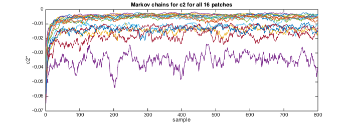
Visual inspection of the Markov chains suggests that they converged to a stationary distribution after 100-200 samples. The length of the Markov chains and of the burn-in period can be modified through the variables "param_model.EST.Nmc" and "param_model.EST.Nbi".

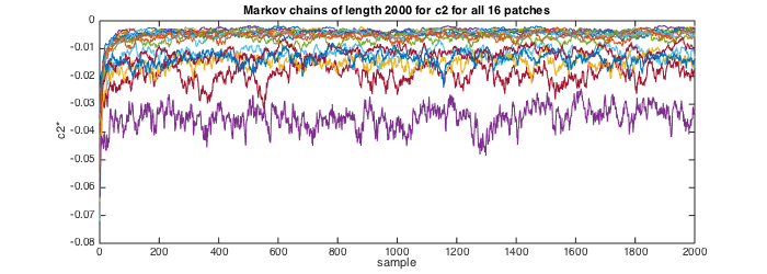
% Sample chains of length 2000 samples
param_model.EST.Nmc=2000;
% Do not use the first 1000 samples in the computation of the Bayesian estimators
param_model.EST.Nbi=1000;
% perform estimation
[estc2,MCc2,~,~,estc1] = est_bayes_mvmfa(lxft,param_model,[1 1]);
% Plot the Markov chains for c2 for all 16 patches
figure(2);clf; set(gcf,'position',[10 10 700 250]);
plot(MCc2'); title('Markov chains of length 2000 for c2 for all 16 patches');xlabel('sample');ylabel('c2*');
Sz_chains=size(MCc2)
estc2
estc1

Sz_chains =
          16        2000
estc2 =
   -0.0035   -0.0039   -0.0054   -0.0047
   -0.0044   -0.0113   -0.0145   -0.0110
   -0.0038   -0.0190   -0.0340   -0.0135
   -0.0033   -0.0045   -0.0065   -0.0052
estc1 =
    0.6969    0.6973    0.6981    0.6987
    0.6966    0.6971    0.6977    0.6982
    0.6961    0.6965    0.6973    0.6978
    0.6957    0.6963    0.6972    0.6976

When the Markov chains are not stored and output, i.e. param_model.EST.MEMSAVE = 0; the posterior vairance of the estimates (i.e., the sample variance of the MCM chains) is output instead.

% do not store MCM chains
param_model.EST.MEMSAVE = 1;
[estc2,PostVar_c2,estc20,PostVar_c20,estc1,PostVar_c1,estc10,PostVar_c10,estSAR,PostVar_SAR] = est_bayes_mvmfa(lxft,param_model,[1 1]);
% Posterior variance for c2
PostVar_c2

PostVar_c2 =
   1.0e-04 *
    0.0068    0.0087    0.0102    0.0101
    0.0061    0.0455    0.0476    0.0580
    0.0074    0.0907    0.1898    0.0636
    0.0060    0.0065    0.0137    0.0091

For univariate estimation of (c2,c1), (i.e., REGU=[0 0], noninformative priors), MAP estimates can in addition be output, as well as the corresponding value of the log-posterior. To do so, the value of the model parameter "param_model.EST.POSTEST" must be set to "1". The MAP estimates and the log-posterior value are output in a structure as the 2nd output argument of "est_bayes_mvmfa.m".

% request MAP estimation and log-posterior evaulation
param_model.EST.POSTEST=1;
% compute univariate estimates for (c2,c1);
REGU=[0 0];
[estc2,STRUCT_MAP,estc20,PostVar_c20,estc1,PostVar_c1,estc10,PostVar_c10,estSAR,PostVar_SAR] = est_bayes_mvmfa(lxft,param_model,REGU);

estMAPc2 = STRUCT_MAP.c2MAP     % MAP estimate for c2
estMAPc1 = STRUCT_MAP.c1MAP     % MAP estimate for c1
logPostVal = STRUCT_MAP.Pt      % log-posterior value corresponding to MAP estimates

PostVar_c2 = STRUCT_MAP.Tc2     % posterior variance of c2 (as above, but now output as structure field)

estMAPc2 =
   -0.0024   -0.0014   -0.0021   -0.0024
   -0.0025   -0.0155   -0.0168   -0.0098
   -0.0008   -0.0281   -0.0434   -0.0142
   -0.0020   -0.0022   -0.0023   -0.0020
estMAPc1 =
    0.6938    0.6715    0.7091    0.6946
    0.6291    0.7059    0.7271    0.7221
    0.6600    0.7351    0.7149    0.6581
    0.6560    0.6853    0.7065    0.7088
logPostVal =
  518.0129  530.9141  530.2712  482.1416
  561.6049  325.9062  279.5146  376.7693
  506.9814  245.1755  120.3001  327.8381
  533.3273  543.6403  334.9808  521.3037
PostVar_c2 =
   1.0e-04 *
    0.0082    0.0040    0.0021    0.0097
    0.0060    0.0860    0.0881    0.0567
    0.0016    0.2119    0.2707    0.0476
    0.0051    0.0079    0.0117    0.0026

Bayesian estimation of multifractal parameters: Output structures

Contents

Synthetic image data

Optional outputs of data preprocessing function "preproc_data_mvmfa.m"

Outputs of Bayesian estimator / Gibbs sampler "est_bayes_mvmfa.m"