Tutorial on the selection of the value for the integral scale

In this tutorial, we will illustrate how the choice of the value for the number of integral scales, which is a model parameter that is assumed to be provided by the user, can be guided by means of the maximum (log-)posterior value attained by the model.

The number of integral scales is defined as the data length divided by the decorrelation length.

Preliminaries and input data
Scaling and correlation analysis
Bayesian model fit analysis
Comparison of estimates obtained for different integral scale values

Preliminaries and input data

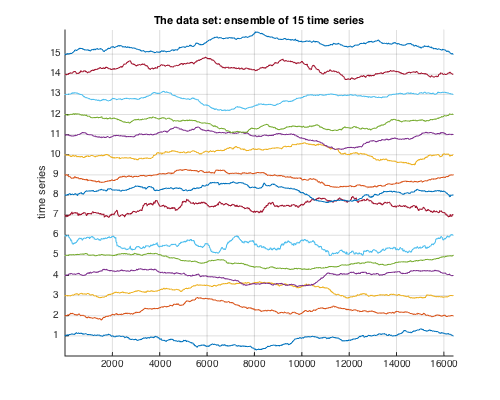
The data under analysis is given by a realization of 15 multifractal time series (N=2^14) with controlled multifractal properties and integral scale. For the first 5 time series, (c1,c2)=(0.7,-0.02), for the next 5 time series, (c1,c2)=(0.7,-0.04), and for the last 5 time series, (c1,c2)=(0.7,-0.01). The number of integral scales is 2^7 for all series (i.e., the decorrelation length is N/2^7=2^7 samples).

% Add the path to toolbox
clear all; clc;
pth=which('est_bayes_mvmfa');if ispc; ii=strfind(pth,'\');else;ii=strfind(pth,'/');end;pth=pth(1:ii(end));addpath(genpath(pth));
% Load synthetic data and theoretical values for c2
load('mrw14_IS.mat');

% Plot the data
zdata=zscore(data')/4;
figure(10);clf;hold on;set(gcf,'position',[10 500 500 400]);
for k=1:size(data,1);LS{k}=num2str(k);plot(zdata(:,k)+k-zdata(1,k));end
grid on;set(gca,'xlim',[1 N]);set(gca,'ylim',[0 16.2]);title('The data set: ensemble of 15 time series');ylabel('time series');%legend(LS);
set(gca,'ytick',[1:15]);set(gca,'yticklabel',[1:15]);

% Multifractal analysis parameters
Nwt = 2;    % number of vanishing moments of wavelet (Daubechies)
gamint = 0; % fractional integration parameter for wavelet leaders
j1=2;       % scaling range lower cutoff
j2=6;       % scaling range upper cutoff

% Data handling parameters
sw=N;  % time window size (here, the entire time series)
dsw=0*sw;       % overlap of windows (here, none)

Scaling and correlation analysis

It can be useful to investigate the linear behavior with scales j of the first and second log-cumulants C1(j) and C2(j). For multifractal cascade processes with a decorrelation length shorter than the data length, C2(j) should saturate at 0 as soon as j>=J, where 2^J is the decorrelation length. As can be seen in the following plot, this is however far from obvious to decide on (remember that the decorrelation length of the data analyzed here is 2^7, yet it is hard to infer this value from the behavior of C2(j)).

% compute mean and variances of log-leaders for all scales (for scaling
% investigation only)
[lxft,pd0,data0,pdata] = preproc_data_mvmfa(data,sw,dsw,1,log2(N)-3,Nwt,gamint);

% plot C1(j) and C2(j) as a function of scale j (overlay of all data
% components)
figure(1);clf; set(gcf,'position',[10 500 1000 300]);
subplot(121);plot(pd0.mV','d-');grid on; xlabel('j = log2(scale)'); ylabel('C1(j)');
subplot(122);plot(pd0.V','d-');grid on; xlabel('j = log2(scale)'); ylabel('C2(j)');

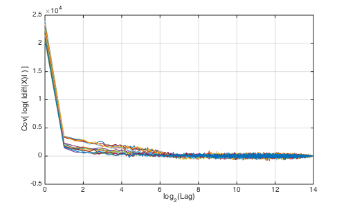
For multifractal cascades, the integral scale (i.e., decorrelation length) is also revealed by the lag for which the autocovariance of the logarithm of the magnitude of the data increments drops to zero. In our example, visual inspection indeed suggests a decorrelation length value somehere between 2^6 and 2^8.

% compute auto-covariance of log-increments of the time series
for i=1:length(CC2); xx(:,i)=xcov(log(abs(diff(data(i,:))))); end
xx=xx(floor(end/2)+1:end,:); tx=1:length(xx);
% plot autocovariance (overlay of all data components)
figure(2);clf;set(gcf,'position',[1000 500 500 300]);
plot(log2(tx),xx);grid on;xlabel('log_{2}(Lag)'); ylabel('Cov[ log( |diff(X)| ) ]');

Bayesian model fit analysis

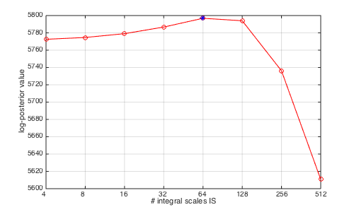
% Data cutting and computation of DWT and DFT for selected scaling range
[lxft,param_data,data0,pdata] = preproc_data_mvmfa(data,sw,dsw,j1,j2,Nwt,gamint); % Data cutting and computation of DWT and DFT

% evaluation of value of log-posterior for different integral scale values
ISL=2.^([2:9]);
for ini=1:length(ISL);
    NII=ISL(ini);     % number of integral scales (default: 1)
    [param_model] = init_model_mvmfa(param_data,'NIScale',NII,'PostVal',1,'Nbi',100,'Nmc',200); % Computation of fixed terms of the spectral density, reparametrization + initialization of prior parameters
    REGU=[0 0]; [eec2,Tc2,ec20tp,Tc20] = est_bayes_mvmfa(lxft,param_model,REGU);
    PV(:,ini)=Tc2.Pt;
end

% find maximizer of log-posterior
[mlogP,ilp] = max(mean(PV));
Est_IS=ISL(ilp),Est_Decorr_Len=N/ISL(ilp)
figure(3);clf;set(gcf,'position',[500 100 500 300]);
plot(log2(ISL),mean(PV),'ro-');hold on; plot(log2(ISL(ilp)),mean(PV(:,ilp)),'b*');hold off;grid on;
set(gca,'xtick',log2(ISL));set(gca,'xticklabel',ISL);xlabel('# integral scales IS');ylabel('log-posterior value');

Est_IS =
    64
Est_Decorr_Len =
   256

Comparison of estimates obtained for different integral scale values

Finally, compute the Bayesian estimates using the selected integral scale value and compare them to Bayesian estimates obtained with far too small and far too large values for the integral scale. The plot also shows the theoretical value for c2, and indicates that the integral scale value selected above is indeed more pertinent than arbitrarily selected (small or large) values.

% compute linear fit (as a baseline reference)
clear ec2; [ec2{1},ec20{1},ec1{1},ec10{1}] = linfit_cp(param_data,0);

% Compute bayesian estimators for different integral scale values
% with estimated number of integral scales
NII=ISL(ilp);
[param_model] = init_model_mvmfa(param_data,'NIScale',NII,'Nbi',500,'Nmc',1500); % Initialize model
    REGU=[0 0]; [ec2{2}(:,1)] = est_bayes_mvmfa(lxft,param_model,REGU); % Compute Bayesian estimators
% with too small number of integral scales
NII=ISL(ilp-1);
[param_model] = init_model_mvmfa(param_data,'NIScale',NII,'Nbi',500,'Nmc',1500); % Initialize model
    REGU=[0 0]; [ec2{2}(:,2)] = est_bayes_mvmfa(lxft,param_model,REGU); % Compute Bayesian estimators
% with too large number of integral scales
NII=ISL(ilp+1);
[param_model] = init_model_mvmfa(param_data,'NIScale',NII,'Nbi',500,'Nmc',1500); % Initialize model
    REGU=[0 0]; [ec2{2}(:,3)] = est_bayes_mvmfa(lxft,param_model,REGU); % Compute Bayesian estimators

% plot estimates
figure(4);clf;tt=1:length(squeeze(CC2(:,:,1)));set(gcf,'position',[10 100 500 300]);
plot(tt,squeeze(CC2(:,:,1)),'r--',tt,squeeze(ec2{1}(:,:,1)),'mx-',tt,squeeze(ec2{2}(:,1)),'ko-',...
    tt,squeeze(ec2{2}(:,2)),'ro-',tt,squeeze(ec2{2}(:,3)),'go-');grid on;set(gca,'xlim',[1 15]);
legend('theo','LF',['IG #is=',num2str(ISL(ilp))],['IG #is=',num2str(ISL(ilp-1))],...
    ['IG #is=',num2str(ISL(ilp+1))]); xlabel('time series'); title('Estimates for c2');

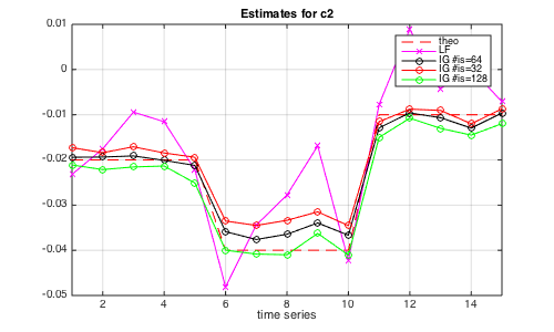
The root-mean-squared-error values for estimates for c2 confirm that the selected value for the integral scale is pertinent.

% compute and display RMSE values
RMSE(1)=sqrt(mean((ec2{1}(:,1)-CC2').^2)); for k=2:4; RMSE(k)=sqrt(mean((ec2{2}(:,k-1)-CC2').^2)); end
disp(' RMSE values:');
disp(['LF          IG IS=',num2str(ISL(ilp)),'    IG IS=',num2str(ISL(ilp-1)),'     IG IS=',num2str(ISL(ilp+1))]);
disp(num2str(round(1e4*RMSE)/1e4))

 RMSE values:
LF          IG IS=64    IG IS=32     IG IS=128
0.0125      0.0026      0.0041      0.0027

Tutorial on the selection of the value for the integral scale

Contents

Preliminaries and input data

Scaling and correlation analysis

Bayesian model fit analysis

Comparison of estimates obtained for different integral scale values