Basic tutorial for Bayesian estimation of multifractal parameters for images

In this brief tutorial, we will step by step perform the multifractal analysis of an image with heterogeneous multifractal properties using Bayesian estimators for the multifractal parameters (log-cumulants) c2 and c1.

Preliminaries and input data
Global analysis of the image
Patch-wise analysis of the image without informative joint priors
Patch-wise analysis of the image with regularizing joint priors
Patch-wise analysis of the image using overlapping patches

Preliminaries and input data

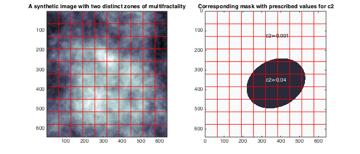
To begin with, set the path to the toolbox, load the data set (situated in this folder), and display it. The image is a realization of a random field with controlled multifractal properties: c1 is constant and equals c1=0.7, and c2 takes the values c2=-0.04 in side an elliptical region, and c2=-0.001 outside.

% add path to toolbox
clear all; clc;
currentpath = cd;addpath([currentpath(1:end-5)]);addpath([currentpath(1:end-5) '/all_tools/']);
% load synthetic data and theoretical values for c2
load('MRWseries640_6.mat'); data=squeeze(data(:,:,5));
C1T=C1;C2T=C2; C1=[0.5 0.9];C2=[-0.05 0]; M2=MASK;M2(MASK==1)=C2T(1);M2(MASK==2)=C2T(2);

% display data and theoretical values for c2
figure(1);clf;set(gcf,'position',[10 500 700 300]);
subplot(121);imagesc(data);colormap bone;
title('A synthetic image with two distinct zones of multifractality');
subplot(122); imagesc(M2); set(gca,'clim',C2); axis tight;
title('Corresponding mask with prescribed values for c2');hold on;
text('string',['c2=',num2str(C2T(1))],'units','normalized','pos',[0.5 0.8]);
text('string',['c2=',num2str(C2T(2))],'color',[1 1 1]-1e-3,'units','normalized','pos',[0.5 0.45]);

Global analysis of the image

We perform the global multifractal analysis of the image. First we need to fix the parameters of the multifractal analysis.

% Multifractal analysis parameters
Nwt = 2;    % number of vanishing moments of wavelet (Daubechies)
gamint = 0; % fractional integration parameter for wavelet leaders
j1=2;       % scaling range lower cutoff
j2=6;       % scaling range upper cutoff

We also need to determine how the image is analyzed, i.e., if we want to estimate multifractal parameters for the global image, or for patches. This is done with the parameters "sw" (horizontal / vertical patch size) and "dsw" (horizontal / vertical overlap between patches)

% data handling parameters
sw=size(data);  % horizontal / vertical image patch size to be analyzed (here, the entire image)
dsw=0*sw;       % overlap of image patches (here, there is only one patch)

These set of parameters (j1,j2,Nwt,gamint,sw,dsw) is all that must be specified by the user. We will see later how to change values of other relevant variables that are automatically set to default values when using only this minimal specification.

The analysis is performed in three steps:

The function "preproc_data_mvmfa" cuts the image into patches according to our specification (sw,dsw), computes the wavelet leaders and the DFT of their logarithm, which is output in "lxft". "lxft" is the input data for the Bayesian estimation algorithms. The second output "param_data" contains parameters associated with "lxft".
The function "init_model_mvmfa" precomputes fixed terms in the Bayesian model and initializes the prior parameters, which are output in "param_model".
The actual Bayesian estimation is performed by the function "est_bayes_mvmfa". It approximates the MMSE estimators for the parameters c2, c1 using a Gibbs sampler (the other outputs will be discussed later).

For comparison, we also compute standard linear regression based estimates for c1 and c2 using the function "linfit_cp".

% Data cutting and computation of DWT and DFT
[lxft,param_data] = preproc_data_mvmfa(data,sw,dsw,j1,j2,Nwt,gamint);
% Precomputation of fixed terms initialization of prior parameters in the Bayesian model
[param_model] = init_model_mvmfa(param_data);

% Bayesian estimation for (c1,c2)
[estc2,~,~,~,estc1] = est_bayes_mvmfa(lxft,param_model);

% Linear regression based estimation (for comparison)
[estc2_lf,ec20{1},estc1_lf,ec10{1}] = linfit_cp(param_data,0);

[estc2 estc2_lf]
[estc1 estc1_lf]

ans =

   -0.0089   -0.0081


ans =

    0.6867    0.6895

Note that the values output by the Bayesian estimator will slightly vary each time the estimator is re-run, despite the fact that the the data remain the same. This is to be expected since the Gibbs sampler is a stochastic algorithm that approximates the posterior expectation by the average of samples drawn at random from the posterior distribution.

Also note that the estimates for c2 make little sense since the image is heterogeneous in c2.

Patch-wise analysis of the image without informative joint priors

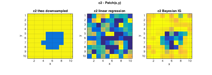
Since the image is heterogeneous in c2, we would like to estimate its multifractal parameters locally, on small patches. We will use square patches of side length 2^6. This is the minimal recommended patch size, which is induced by the dyadic multi-scale analysis underlying the present multifractal analysis algorithms. To accomodate for the small patch size, the scaling range must be reduced also.

L = 2^6; sw = [L L]; % size of patch to be analyzed (sw <= image size)
dsw=0*sw;           % no overlap
j1=1;
j2=2;
% display the patches on the original image
figure(1);subplot(121);hold on; for n1=1:9;plot(L*n1*[1 1],[0 640],'r');plot([0 640],L*n1*[1 1],'r');end
subplot(122);hold on; for n1=1:9;plot(L*n1*[1 1],[0 640],'r');plot([0 640],L*n1*[1 1],'r');end

The lines of code for performing the estimation are identical to above. The Bayesian estimation is performed with a non-informative inverse Gamma (IG) prior for c2, and a non-informative Normal prior (N) for c1.

% Data cutting and computation of DWT and DFT
[lxft,param_data] = preproc_data_mvmfa(data,sw,dsw,j1,j2,Nwt,gamint);
% Precomputation of fixed terms initialization of prior parameters in the Bayesian model
[param_model] = init_model_mvmfa(param_data);
% Bayesian estimation for (c1,c2) with univariate non-informative priors
[ec2{2},Tc2,ec20tp,Tc20,ec1{2},Tc1,ec10tp,Tc10] = est_bayes_mvmfa(lxft,param_model);

% linear fit (for comparison)
[ec2{1},ec20{1},ec1{1},ec10{1}] = linfit_cp(param_data,0);

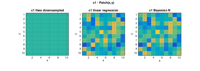
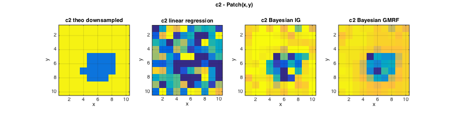
The following plots show that the Bayesian estimator for c2 significantly improves estimation quality over the standard linear regression based estimation.

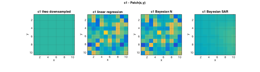
For c1, the estimates for linear regression and Bayesian estimation are identical because the non-informative Normal prior leads to an estimator equivalent to a linear regression.

% Plots
cc0=MASK(L/2:L:end,L/2:L:end);c1=zeros(size(cc0));c2=zeros(size(cc0)); for k=1:length(C1T);c1(cc0==k)=C1T(k);c2(cc0==k)=C2T(k);end;
figure(2);clf; set(gcf,'position',[10 10 700 250]);
subplot(131);imagesc(squeeze(c2));axis image; grid on; caxis(C2); title('c2 theo downsampled');xlabel('x');ylabel('y');
subplot(132);imagesc(squeeze(ec2{1}));axis image; grid on; caxis(C2); title('c2 linear regression');xlabel('x');ylabel('y');
subplot(133);imagesc(squeeze(ec2{2}));axis image; grid on; caxis(C2); title('c2 Bayesian IG');xlabel('x');ylabel('y');
axes('Units','Normal');h = title('c2 - Patch(x,y)');set(gca,'visible','off');set(h,'visible','on');

figure(3);clf; set(gcf,'position',[1000 10 700 250]);
subplot(131);imagesc(squeeze(c1));axis image; grid on; caxis(C1);title('c1 theo downsampled');xlabel('x');ylabel('y');
subplot(132);imagesc(squeeze(ec1{1}));axis image; grid on; caxis(C1); title('c1 linear regression');xlabel('x');ylabel('y');
subplot(133);imagesc(squeeze(ec1{2}));axis image; grid on; caxis(C1); title('c1 Bayesian N');xlabel('x');ylabel('y');
axes('Units','Normal');h = title('c1 - Patch(x,y)');set(gca,'visible','off');set(h,'visible','on');

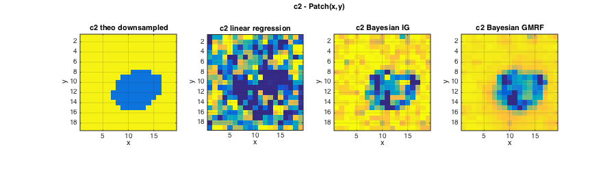
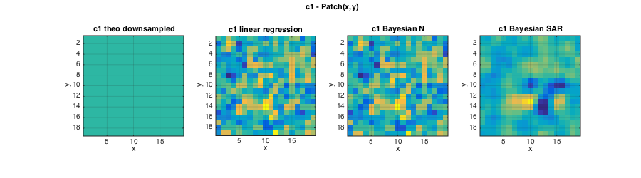
Patch-wise analysis of the image with regularizing joint priors

The estimation performance of the Bayesian estimator for multivariate data, such as a collection of image patches, can be significantly improved by using informative, regularizing joint priors for the parameters c2 and c1 of the data components. The following priors are used for c2 and c1:

The prior for c2 is constructed as a hidden gamma Markov random field (GMRF). For the image patches considered here, a spatial (2D) prior is used. The degree of regularization induced by the prior is determined by hyperparameters that must be specified.

The prior for c1 is a Gaussian-type simultaneous autoregression (SAR) prior. The hyperparameters that tune the degree of regularization are embedded in the Bayesian model and automatically estimated.

Before performing the estimation, we adjust the hyperparameter of the GMRF. The hyperparameter for the 2D GMRF can be changed from the default value as follows:

% adjust regularization parameter for 2D GMRF prior for c2
param_model.EST.GMRF.a = 1.5 * ones(size(param_model.EST.GMRF.a));

The informative priors GMRF and SAR are activated by the additional input [GMRF SAR] to est_bayes_mvmfa, where GMRF and SAR are 1 or 0 (for on or off). For example, [0 0] will perform univariate estimation as above, [1 1] will perform joint estimation using GMRF for c2 and SAR for c1, [1 0] will use the informative (GMRF) prior for c2 and univariate priors for c1, and the combination [0 1] is not implemented.

% Perform joint estimation for (c2,c1) using informative GMRF and SAR priors
REGU=[1 1]; [ec2{3},Tc2,ec20tp,Tc20,ec1{3},Tc1,ec10tp,Tc10] = est_bayes_mvmfa(lxft,param_model,REGU);

The following plots illustrate that the informative GMRF prior further improves the estimation performance for c2, and that now also the Bayesian estimation of c1 clearly improves over linear regression based estimates.

% Plots
figure(2);clf; set(gcf,'position',[10 10 900 250]);
subplot(141);imagesc(squeeze(c2));axis image; grid on; caxis(C2); title('c2 theo downsampled');xlabel('x');ylabel('y');
subplot(142);imagesc(squeeze(ec2{1}));axis image; grid on; caxis(C2); title('c2 linear regression');xlabel('x');ylabel('y');
subplot(143);imagesc(squeeze(ec2{2}));axis image; grid on; caxis(C2); title('c2 Bayesian IG');xlabel('x');ylabel('y');
subplot(144);imagesc(squeeze(ec2{3}));axis image; grid on; caxis(C2); title('c2 Bayesian GMRF');xlabel('x');ylabel('y');
axes('Units','Normal');h = title('c2 - Patch(x,y)');set(gca,'visible','off');set(h,'visible','on');
figure(3);clf; set(gcf,'position',[700 10 900 250]);
subplot(141);imagesc(squeeze(c1));axis image; grid on; caxis(C1);title('c1 theo downsampled');xlabel('x');ylabel('y');
subplot(142);imagesc(squeeze(ec1{1}));axis image; grid on; caxis(C1); title('c1 linear regression');xlabel('x');ylabel('y');
subplot(143);imagesc(squeeze(ec1{2}));axis image; grid on; caxis(C1); title('c1 Bayesian N');xlabel('x');ylabel('y');
subplot(144);imagesc(squeeze(ec1{3}));axis image; grid on; caxis(C1); title('c1 Bayesian SAR');xlabel('x');ylabel('y');
axes('Units','Normal');h = title('c1 - Patch(x,y)');set(gca,'visible','off');set(h,'visible','on');

Patch-wise analysis of the image using overlapping patches

We finally analyze the image using patches of side length 2^6 that overlap 50% horizontally and vertically.

L = 2^6; sw = [L L];  % size of patch to be analyzed (sw <= image size)
dsw=0.5*sw;           % 50% horizontal and vertical overlap between patches

The lines of code for performing the estimation are identical to above. For comparison, we will use non-informative inverse Gamma (IG) and Normal (N) priors, as well as regularizing GMRF and SAR priors.

% Data cutting and computation of DWT and DFT
[lxft,param_data] = preproc_data_mvmfa(data,sw,dsw,j1,j2,Nwt,gamint);
% Precomputation of fixed terms initialization of prior parameters in the Bayesian model
[param_model] = init_model_mvmfa(param_data);

% Bayesian estimation for (c1,c2) with univariate non-informative priors
REGU=[0 0]; [ec2{2},Tc2,ec20tp,Tc20,ec1{2},Tc1,ec10tp,Tc10] = est_bayes_mvmfa(lxft,param_model,REGU);

% Adjust regularization parameter for 2D GMRF prior for c2 and perform
% Bayesian joint estimation for (c2,c1) using informative GMRF and SAR joint priors
param_model.EST.GMRF.a=1.5*ones(size(param_model.EST.GMRF.a));
REGU=[1 1]; [ec2{3},Tc2,ec20tp,Tc20,ec1{3},Tc1,ec10tp,Tc10] = est_bayes_mvmfa(lxft,param_model,REGU);

% linear fit (for comparison)
[ec2{1},ec20{1},ec1{1},ec10{1}] = linfit_cp(param_data,0);